The purpose of this article is to realize gradient descent algorithm for univariate linear regression in Python. We first briefly show the mathematics of the algorithm and then the code in Python to realize gradient descent method.
The cost function that will be used is mean square error (MSE). Let’s define some notations that will be used later.


The purpose of gradient descent is to keep updating our parameters, 


And similarly,


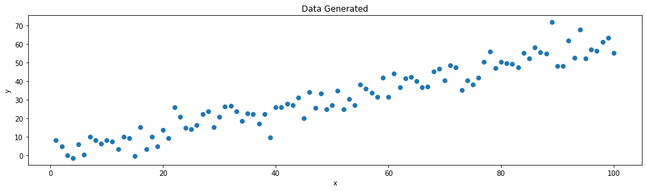
To generate some data, we let x be a series from 1 to 100 with steps of 1 and 

import numpy as np
import matplotlib.pyplot as plt

np.random.seed(2021)
x = np.arange(1, 101, 1)
y = 0.6*x + 0.2 + np.random.normal(scale=5,size=len(x))

f, ax = plt.subplots(figsize=(16,4))
plt.title("Data Generated")
ax.scatter(x, y)
plt.xlabel("x")
plt.ylabel("y")
plt.show()
The generated data are plotted.
Now, we need to define some functions for our gradient descent algorithm.
# Hypothesis
def h(x,t0,t1):
    x_ = np.array([np.ones(len(x)), x]).T
    y = np.matmul(x_, np.array([t0,t1]))
    return y

# Cost Function
def cost_f(y, y_hat):
    diff = y_hat - y
    diff_sq = np.power(diff,2)
    cost = 0.5 * np.mean(diff_sq)
    return cost

# Gradient Function
def t0_grad_f(t0,t1,x,y):
    diff = t0 + t1*x - y
    t0_grad = np.mean(diff)
    return t0_grad

def t1_grad_f(t0,t1,x,y):
    diff = (t0 + t1*x - y) * x
    t1_grad = np.mean(diff)
    return t1_grad

# Gradient Descent
def grad_desc(x,y,t0=0,t1=0,lr=0.0001):
    cost_list = []
    cost = 1e99
    while True:
        t0_grad = t0_grad_f(t0=t0,t1=t1,x=x,y=y)
        t1_grad = t1_grad_f(t0=t0,t1=t1,x=x,y=y)
        t0 = t0 - lr*t0_grad
        t1 = t1 - lr*t1_grad
        y_hat = h(x=x, t0=t0, t1=t1)
        cost_new = cost_f(y, y_hat)
        cost_list.append(cost_new)
        if cost_new > cost:
            break
        cost = cost_new
    return [t0,t1], cost_list
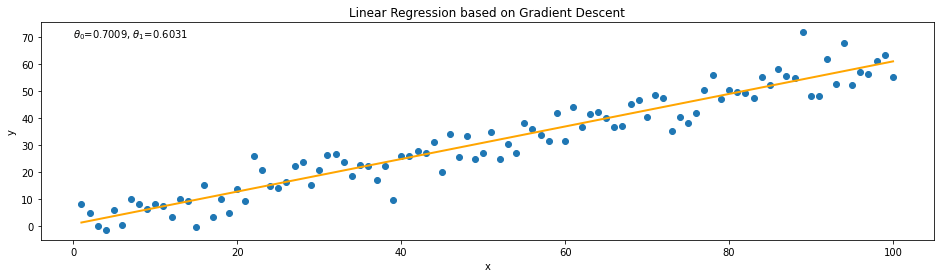
Then, we can run the function and plot our fitted model:
# Run gradient descent
coef_, _ = grad_desc(x=x, y=y)

# Fit data using GD results
y_hat = coef_[0] + x*coef_[1]

# Plot the data and model
f, ax = plt.subplots(figsize=(16,4))
plt.title("Linear Regression based on Gradient Descent")
plt.text(x=0, y=70, s=r"$\theta_0$={}, $\theta_1$={}".format(np.round(coef_[0],4),np.round(coef_[1],4)))
plt.xlabel("x")
plt.ylabel("y")
ax.scatter(x,y)
ax.plot(x,y_hat, color='orange', lw=2)
plt.show()
Notes:
- For linear gradient descent problem, the initial parameter
- The learning rate needs to be set carefully. Large learning rate will cause a divergent result while small learning rate will take long time to converge.
