Multivariate Linear Regression with Gradient Descent

In this article, I will try to extend the material from univariate linear regression into multivariate linear regression (mLR). In mLR, n features are collected for each observation, and is now also a vector of dimension n+1 where is the intercept, or the coefficient for an arbitrary feature of x with all values equal to 1. The hypothesis/model is now written as:

And let’s use to denote the feature of observation.

To realize gradient descent, let’s try to obtain the gradient for our cost function which is now written as:

.

For each feature j and its corresponding coefficient , the gradient will be:

The dataset that we will be using for multivariate linear regression is the fish market data from Kaggle.com. The dataset contains 159 observations with 7 features.

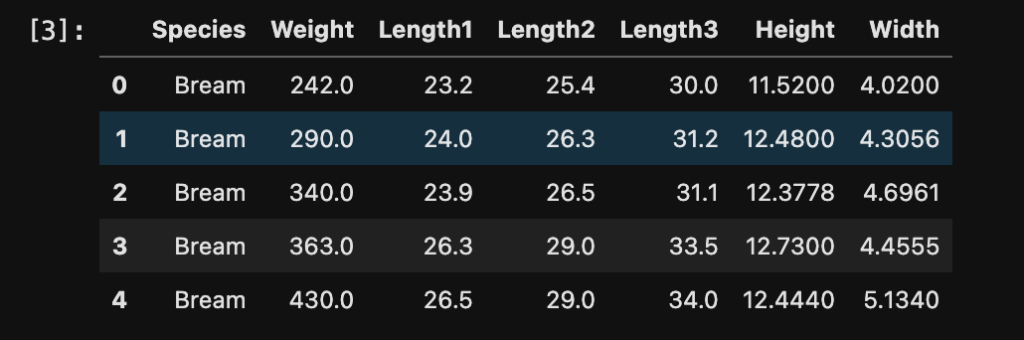
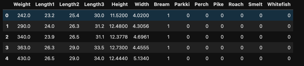
For illustration purpose, we will convert Species into features by one-hot coding. In this dataset, the correlation between variables are large, meaning not all features should be included in our model. But we can still use all features for showing multivariate gradient descent process. To import and convert the dataset:

import pandas as pd
# Import Data
df = pd.read_csv("Fish.csv")
# Get dummy variables for species
dummies = pd.get_dummies(df['Species'])
# Join data together
data = df.join(dummies).drop("Species", axis=1)
data.head()

Let’s choose Weight as our target variable. Before building the model, let’s create some functions for gradient descent process.

# Hypothesis
def h(df,theta=None):
    if theta is None:
        theta_ = np.ones(df.shape[1]+1)
    else:
        theta_ = theta
    df_ = df.copy()
    y = df_.dot(theta_)
    return y
# Define cost function
def cost_f(y_hat, y):
    diff = y_hat - y
    cost = 0.5*(diff.pow(2).mean())
    return cost
# Calculate gradient
def gradient(X, y, theta=None):
    n = X.shape[1] + 1
    if theta is None:
        theta_ = np.ones(X.shape[1] + 1)
    else:
        theta_ = theta
    if len(theta_) != n:
        print("Dimension of theta: {} does not match {} features in X.".format(len(theta), n))
    else:
        X_ = X.copy()
        intercepts = np.ones(df.shape[0])
        X_.insert(loc=0,column = "Intercept",value=pd.Series(intercepts))
        grads = []
        for j in range(n): # iterate j from 0 to n
            diff = (h(X_, theta=theta_) - y)*X_.iloc[:,j]
            grad = diff.mean()
            grads.append(grad)
    out = np.array(grads)
    return out
# Update theta with gradient descent
def gradient_descent(X, y, theta=None, alpha=0.0003):
    cost = 1e99
    cost_list = []
    
    if theta is None:
        theta_ = np.ones(X.shape[1] + 1)
    else:
        theta_ = theta
    df = X.copy()
    intercepts = np.ones(df.shape[0])
    df.insert(loc=0,column = "Intercept",value=pd.Series(intercepts))
    from IPython.display import display, clear_output
    i=0
    while True:
        grad = gradient(X=X, y=y, theta=theta_)
        theta_ -= alpha * grad
        y_hat = h(df, theta_)
        cost_new = cost_f(y_hat, y)
        i+=1
        display("Iteration: {}, cost: {}".format(i, cost_new))
        clear_output(wait=True)
        if cost_new > cost:
            break
        cost = cost_new
        cost_list.append(cost)
        
    return theta_, cost_list

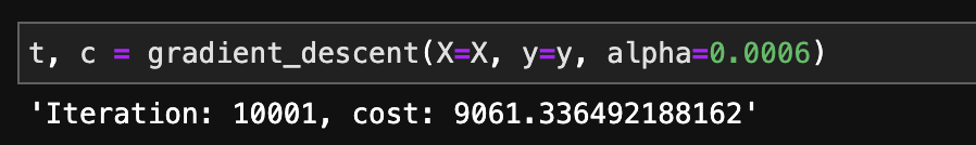
In the Python code above, the iteration of gradient descent will stop when the new cost is less than previous cost by a pre-defined tolerance or max iteration is reached. The result is shown below:

The cost vs iteration is plotted as follows:

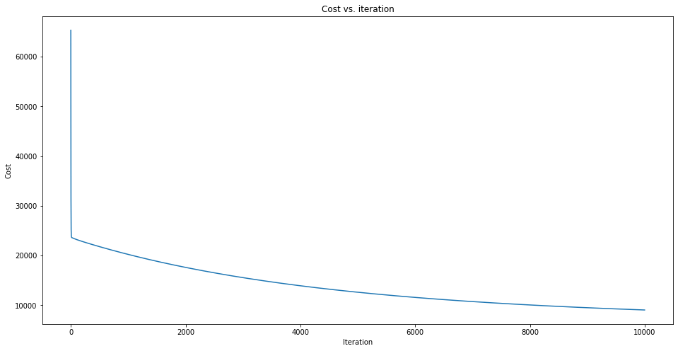
A sharp decrease is observed at the beginning of the iteration and cost keeps decreasing as the algorithm iterates. Given enough time for iteration, the cost function will converge to a smaller value and the optimal can be obtained then.

Some quick notes:
1. For faster result, we can use normal equation to solve for optimal and the equation is expressed as follows:

2. According to linear analysis assumptions, the features selected should be independent of each other. Again, this is an illustration of multivariate linear regression based on gradient descent. Feature selection is not discussed in this article but should always be considered when working with real data and real model.
3. Polynomial regression can be achieved by adding columns that equal to some existing columns to the power of degree d. Interaction effects can also be explored by multiplying two or more columns together.
4. For faster convergence, features should be scaled.