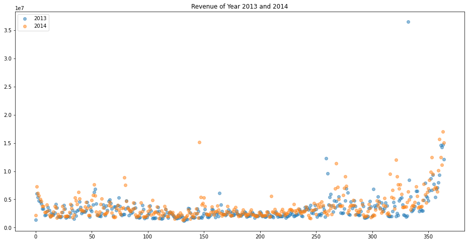
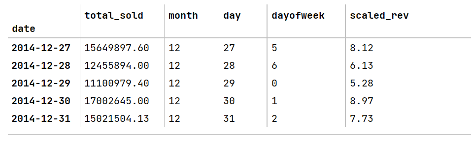
Using the same data set as in Part I, let’s explore some methods to apply linear regression for time-series data. Our data looks like this:
To model the data using linear regression, we need to convert date and time into features and scale the revenue into the appropriate range.
df_daily['month'] = df_daily.index.month
df_daily['day'] = df_daily.index.day
df_daily['dayofweek']=df_daily.index.weekday

from sklearn.preprocessing import RobustScaler
transformer = RobustScaler().fit(df_daily['total_sold'].to_numpy().reshape(-1,1))
df_daily['scaled_rev'] = transformer.transform(df_daily['total_sold'].to_numpy().reshape(-1,1))
And now our dataset looks like this:
Note that we can observe some increase in revenue at the beginning and end of a year, so the intuition suggests possible polynomial linear models. To compare, let’s use simple linear regression as a baseline and then the polynomial model. I will use the data of 2013 and 2014 for training and 2015 for testing.
Direct Fit
poly = PolynomialFeatures(degree = 1)
X = poly.fit_transform(df_daily.drop(['total_sold','scaled_rev','is_holiday'], axis=1))
X_ = pd.DataFrame(X)
X_ = X_.join(df_daily['is_holiday'].reset_index()).set_index('date')
df_train = X_.loc[:'2014-12-31']
df_test = X_.loc['2015-01-01':]

x_train = X_.loc[:'2014-12-31']
y_train = df_daily.loc[:'2014-12-31']['scaled_rev']
x_test = X_.loc['2015-01-01':]
y_test = df_daily.loc['2015-01-01':]['scaled_rev']


LinModel = LinearRegression()
LinModel.fit(x_train, y_train)
pred = LinModel.predict(x_test)
y_hat = transformer.inverse_transform(pred.reshape(-1,1))
np.sqrt(mean_squared_error(y_test, y_hat))
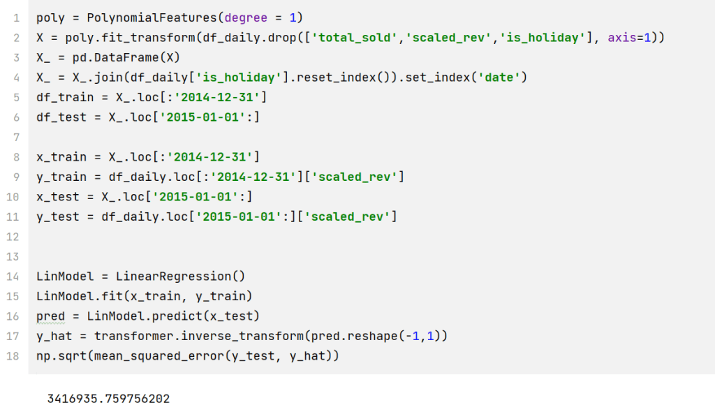
The RMSE of a simple linear model is 3,416,935. Now, let’s use the polynomial model. Note that I choose Ridge regression instead of simple linear regression. A regularized model could prevent overfitting by adding a penalized term to the cost function.
poly = PolynomialFeatures(degree = 3)
X = poly.fit_transform(df_daily.drop(['total_sold','scaled_rev','is_holiday'], axis=1))
X_ = pd.DataFrame(X)
X_ = X_.join(df_daily['is_holiday'].reset_index()).set_index('date')
df_train = X_.loc[:'2014-12-31']
df_test = X_.loc['2015-01-01':]

x_train = X_.loc[:'2014-12-31']
y_train = df_daily.loc[:'2014-12-31']['scaled_rev']
x_test = X_.loc['2015-01-01':]
y_test = df_daily.loc['2015-01-01':]['scaled_rev']


LinModel = Ridge(alpha=0.1)
LinModel.fit(x_train, y_train)
pred = LinModel.predict(x_test)
y_hat = transformer.inverse_transform(pred.reshape(-1,1))
np.sqrt(mean_squared_error(y_test, y_hat))
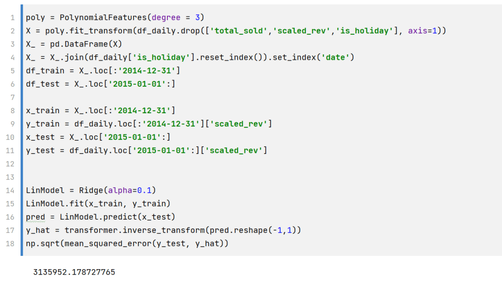
The RMSE decreases to 3135952, which is better than the simple linear model.
Feature Engineering
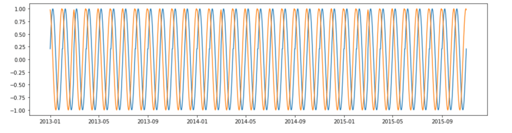
On second thought, the last day of a month and the first day of a month are next to each other. So let’s use periodic functions, e.g. sin() and cos(), to denote days within a month. And we can do the same for weekdays and months within a year.
df_fe = df_daily.copy()
d_sin = np.sin(df_fe['day'].mul(2 * np.pi).div(30))
d_cos = np.cos(df_fe['day'].mul(2 * np.pi).div(30))
plt.figure(figsize=(16, 4))
plt.plot(d_sin)
plt.plot(d_cos)
plt.show()

w_sin = np.sin(df_fe['dayofweek'].mul(2 * np.pi).div(7))
w_cos = np.cos(df_fe['dayofweek'].mul(2 * np.pi).div(7))
m_sin = np.sin(df_fe['month'].mul(2*np.pi).div(12))
m_cos = np.cos(df_fe['month'].mul(2*np.pi).div(12))
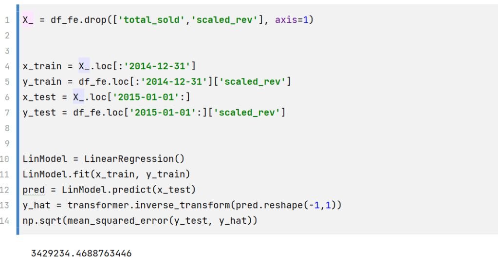
Now, let’s feed the data through a linear regression model.
X_ = df_fe.drop(['total_sold','scaled_rev'], axis=1)
x_train = X_.loc[:'2014-12-31']
y_train = df_fe.loc[:'2014-12-31']['scaled_rev']
x_test = X_.loc['2015-01-01':]
y_test = df_fe.loc['2015-01-01':]['scaled_rev']


LinModel = LinearRegression()
LinModel.fit(x_train, y_train)
pred = LinModel.predict(x_test)
y_hat = transformer.inverse_transform(pred.reshape(-1,1))
np.sqrt(mean_squared_error(y_test, y_hat))
Now, we can also try polynomial features on the engineered dataset.
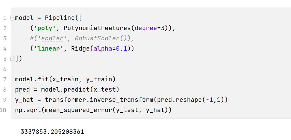
The method of transforming days and months into periodic functions works best when certain seasonality exists. For this dataset, such seasonality does not exist based on our previous analysis. Therefore, we only demonstrate the method but will not dive deep into such an engineered model.
