In this part, let’s build an LSTM model for the sales revenue data. Long short temporary model is developed on the basis of Recurrent Neural Network to improve its performance in NLP by retaining some information from “long” past data. Due to its capability of processing sequence data, LSTM can also be used to model time series data.
More information and examples about LSTM can be found on Tensorflow tutorials.
Let’s jump into the case.
Import, Clean the Data
df_raw['total_sold'] = df_raw["item_price"]*df_raw['item_cnt_day']
df_raw['date']=pd.to_datetime(df_raw['date'], dayfirst=True)
df_raw.set_index('date', inplace=True)
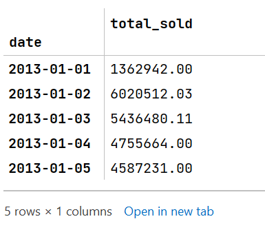
df_daily = df_raw[['total_sold']].resample('D').sum()
df_daily.head()
Getting Data Ready for Training
After importing necessary modules, let’s create a function that returns our training and testing set. We are using the values from previous lookback days to predict the value of day lookback+1.
from sklearn.preprocessing import StandardScaler
from sklearn.metrics import mean_squared_error
from tensorflow.keras.models import Sequential
from tensorflow.keras.layers import LSTM, Dropout, Dense

def gen_xy(y, lookback=10):
    x, targets = [],[]
    n = len(y)
    for i in range(n-lookback):
        x_ = y[i:i+lookback]
        y_ = y[i+lookback]
        x.append(x_)
        targets.append(y_)
    x = np.array(x)
    targets = np.array(targets)
    return x, targets
For training and testing, I will use a split ratio of 0.75. The following code shows how the dataset is partitioned:
split_ratio = 0.75

scaler = StandardScaler().fit(df_daily)
y = scaler.transform(df_daily)
x, targets = gen_xy(y)
train_len = int(split_ratio * x.shape[0])
x_train = x[:train_len]
y_train = targets[:train_len]
x_test = x[train_len:]
y_test = targets[train_len:]
Build and Train LSTM Neural Network
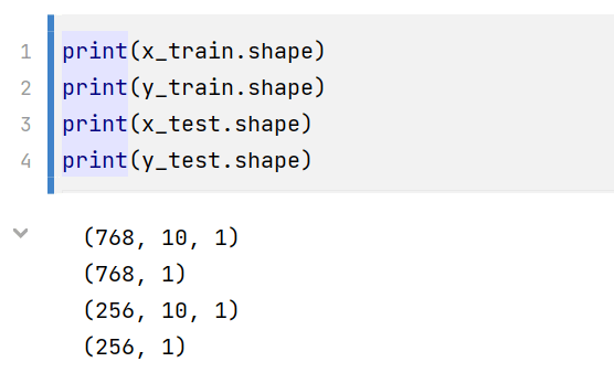
The x_train and y_test are already shaped in (n_observations, time_steps, n_features) so we can directly feed the dataset into LSTM with input_shape = (time_steps, n_features). And here is the code:
model = Sequential()
model.add(LSTM(16,input_shape=(10,1), return_sequences=True, activation='relu'))
model.add(Dropout(0.1))
model.add(LSTM(4, activation='relu'))
model.add(Dropout(0.1))
model.add(Dense(1))
model.compile(loss='mse', optimizer='adam')
Then, we can train and test the model.
EPOCHS = 20
model.fit(x_train, y_train, epochs=20, verbose=1)
y_hat = model.predict(x_test)
y_pred = scaler.inverse_transform(y_hat)
print("RMSE: ", np.sqrt(mean_squared_error(y_test, y_pred)))
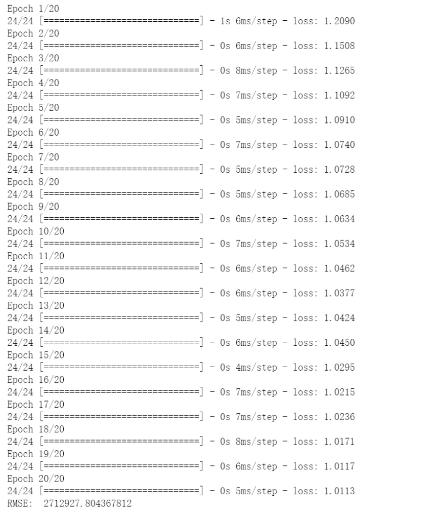
It is performing better than our linear regression model with RMSE of 2,712,927. Let’s visualize the results:
# join actual and predicted values
idx = df_daily.index[-len(y_pred):]
predicts = pd.DataFrame(y_pred, index=idx, columns=['predicts'])
y_plot = df_daily.join(predicts)

# visualization
f, ax = plt.subplots(figsize=(16,8))
ax.set_title('LSTM Prediction')
ax.plot(y_plot['total_sold'], alpha=0.75,label='Actual')
ax.plot(y_plot['predicts'], label='Prediction')
ax.legend(loc='upper left')
plt.show()
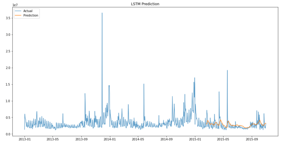
The predictions follow the overall trend of the data well with some lag. Keep in mind that the model is only trained with 20 epochs and no hyper-parameter tuning is performed. Therefore, we are expecting to see further decrease in final RMSE when the model is properly tuned.
