- PLEASE DO NOT USE THE MODEL IN THIS ARTICLE FOR TRADING OR USE IT AT YOUR OWN RISK. LIVE MARKETS ARE VERY COMPLICATED AND THE MODEL IN THIS ARTICLE WILL NOT GUARANTEE PROFITS.
In this article, let’s try to utilize LSTM techniques to predict the price of bitcoin. Unlike what we have done for the sales data, predicting the price of bitcoin, or any other types of cryptocurrencies as well as stocks, requires carefully handling of the data. For the previous sales data modeling, as the data is tested to be stationary with no trend present, we can standardize the data using the entire training set. However, using the same technique when dealing with stock/cryptocurrency prices could lead to intaking too much past information into the model. Therefore, in this article, to model the price of bitcoin, let’s try to standardize the data batch-by-batch.
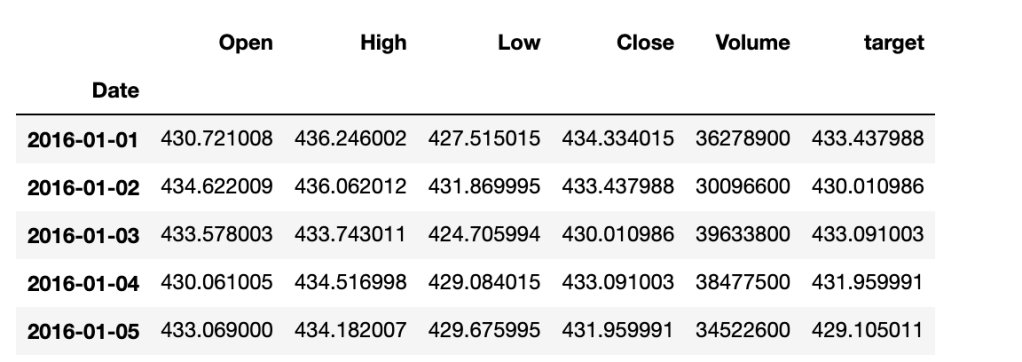
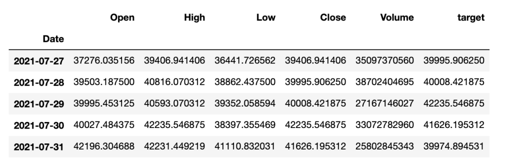
To fetch the price data of bitcoin, I will use yfinance package. Our target will be the close price of next day (


import pandas as pd
import numpy as np
import yfinance as yf

# Fetch history data
Ticker = yf.Ticker('BTC-USD')
history = Ticker.history(start='2016-01-01', end='2021-08-01')
history.drop(['Dividends', 'Stock Splits'], axis=1, inplace=True)

# Create a the target column
history['target'] = history['Close'].shift(-1)
history = history.dropna()

history.head()
Now, let’s create a function to generate our X and y datasets for training and testing. Keep in mind that since we are going to standardize batch-by-batch, it is more convenient to also generate reference datasets so that we can use them to inverse our predictions.
def xy_gen(x,y,lookback=14, split_ratio=0.75):
    x_ = []
    y_ = []
    y_ref = []
    n = len(y)
    for i in range(n-lookback):
        x_t = x.iloc[i:i+lookback,]
        y_ref.append(x_t['Close'])
        y_t = y.iloc[i+lookback-1,]
        y_t = (y_t - x_t['Close'].mean())/x_t['Close'].std()
        x_t = (x_t - x_t.mean())/x_t.std()
        x_.append(x_t)
        y_.append(y_t)

    n_train = int(n*split_ratio)
    x_train = x_[:n_train]
    y_train_ref = y_ref[:n_train]
    y_train = y_[:n_train]
    x_test = x_[n_train:]
    y_test = y_[n_train:]
    y_test_ref = y_ref[n_train:]

    return np.array(x_train), np.array(y_train), np.array(x_test), np.array(y_test), y_train_ref, y_test_ref

x_train, y_train, x_test, y_test, y_train_ref, y_test_ref = xy_gen(history.drop('target',axis = 1), history[['target']])
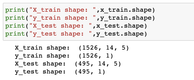
Let’s check the shape of our generated data.
The next step is to construct an LSTM model for the dataset and feed our data into the model.
from tensorflow.keras.models import Sequential
from tensorflow.keras.layers import Dropout, Dense, LSTM
model = Sequential()
model.add(LSTM(32,input_shape=(14,5), activation='relu', return_sequences=True))
model.add(Dropout(0.2))
model.add(LSTM(16, activation='relu',return_sequences=True))
model.add(LSTM(16, activation='relu',return_sequences=True))
model.add(Dropout(0.2))
model.add(LSTM(4))
model.add(Dense(1))
model.compile(loss='mse', optimizer='adam')
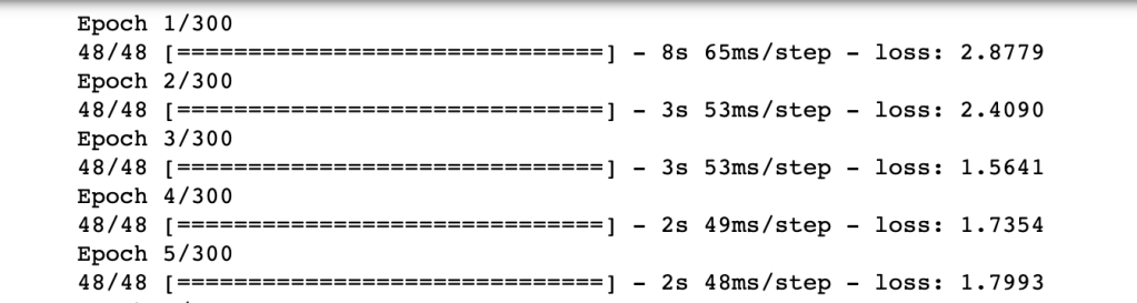
model.fit(x_train, y_train, epochs=300, verbose=1)
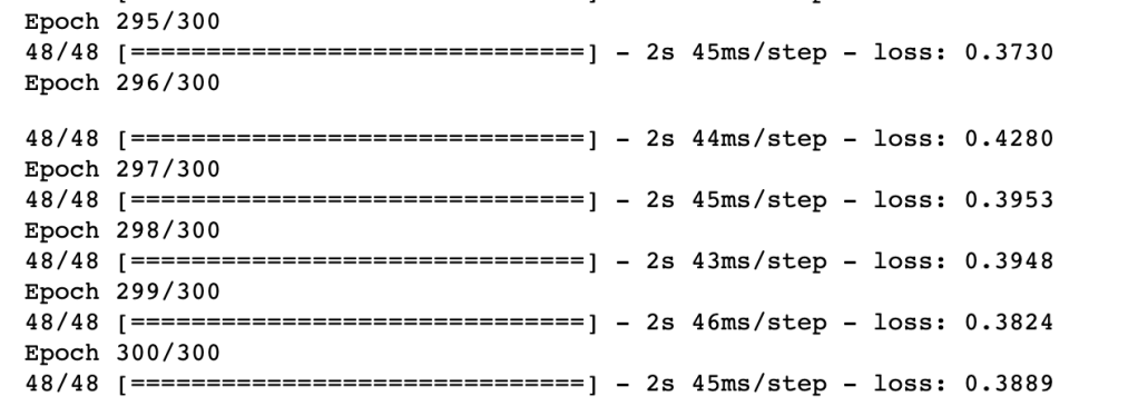
Now, we have our model and let’s see how the model performs with test data.
y_pred = model.predict(x_test)

f, ax = plt.subplots(figsize=(16,4))
plt.title('Non-inversed Results')
ax.plot(y_test, label='Actual')
ax.plot(y_pred, label='Predict')
plt.legend()
plt.show()
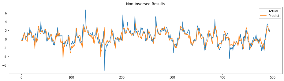
The prediction follows the trend of actual somehow. It actually looks good to me. Let’s see the actual prediction by inverting the values. Let’s create an inverse function first.
def inverse_y(y, ref):
    y_inv = []
    for i in range(len(y)):
        mean = np.mean(ref[i])
        std = np.std(ref[i])
        y_i = (y[i]*std)+mean
        y_inv.append(y_i)
    return np.array(y_inv)
# inverse
y_pred_inv = inverse_y(y_pred, y_test_ref)

# create a DataFrame for plotting
idx = history.index[-len(y_test_inv):]
df_pred = pd.DataFrame(y_pred_inv, index=idx)

# Plot
from matplotlib.ticker import (MultipleLocator, AutoMinorLocator)

f, ax = plt.subplots(nrows=2,figsize=(32,16))
ax[0].set_title('Close Price v.s. Targets v.s. Predicts', fontsize=25)
ax[0].plot(history['Close'][-len(df_pred):], color='blue', label='Close', lw=5)
ax[0].xaxis.set_minor_locator(MultipleLocator(5))
ax[0].grid(True, which = 'minor', axis='x')
ax[0].legend(loc='upper left', fontsize=20)
ax[1].plot(history['target'][-len(df_pred):], color='orange', label='target', lw=5)
ax[1].xaxis.set_minor_locator(MultipleLocator(5))
ax[1].grid(True, which = 'minor', axis='x')
ax[1].plot(df_pred, alpha=0.5, label = 'Predicts', color='green',lw=5)
ax[1].legend(loc='upper left', fontsize=20)
plt.show()
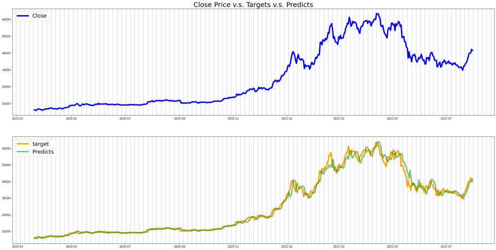
The predicted price follows the trend of our targets well but there are lags observed. The calculated RMSE of the test set is approximately 2,150.
