ARIMA is known for its effectiveness in modeling time series data. In this section, we will try to fit the data using an ARIMA model. Theoretically, the parameters, (p, q), of an ARIMA(p, d, q) is selected using partial autocorrelation and autocorrelation coefficients. The parameter of d implies the number of times we take differences on the data such that the data reach stationarity.
In earlier analysis, we have already used Augmented Dickey Fuller test to show that the data is already stationary. Thus, the d parameter will be equal to 0. The partial autocorrelation plot and autocorrelation plot of the dataset is drawn as follows:
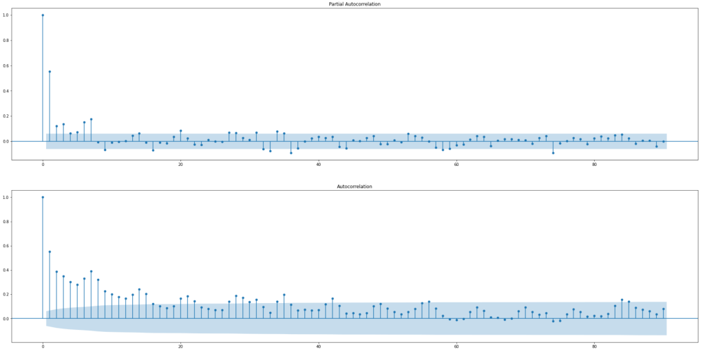
According to the plots, we can let p=7 and q=16. Let’s use the data in 2013 and 2014 as our training set and the data in 2015 as our testing set. First, let’s clean the dataset and then we can start building the model.
import pandas as pd
# Read Dataset
df_raw = pd.read_csv('sales.csv')

# Convert datatypes
df_raw['date']=pd.to_datetime(df_raw['date'], dayfirst=True)
df_raw = df_raw.sort_values("date")
df_raw['total_sold'] = df_raw['item_price']*df_raw['item_cnt_day']
df_raw.set_index('date', inplace=True)

# Calculate daily revenue
df_daily = df_raw['total_sold'].resample('D').sum()
import statsmodels.api as sm

# Split training and testing sets
train = df_daily.loc[:'2014-12-31']
test = df_daily.loc['2015-01-01':]

# Build ARIMA model and show model summary
model = sm.tsa.SARIMAX(train, order=(7,0,16), enforce_stationarity=False)
model_fit = model.fit()
model_fit.summary()
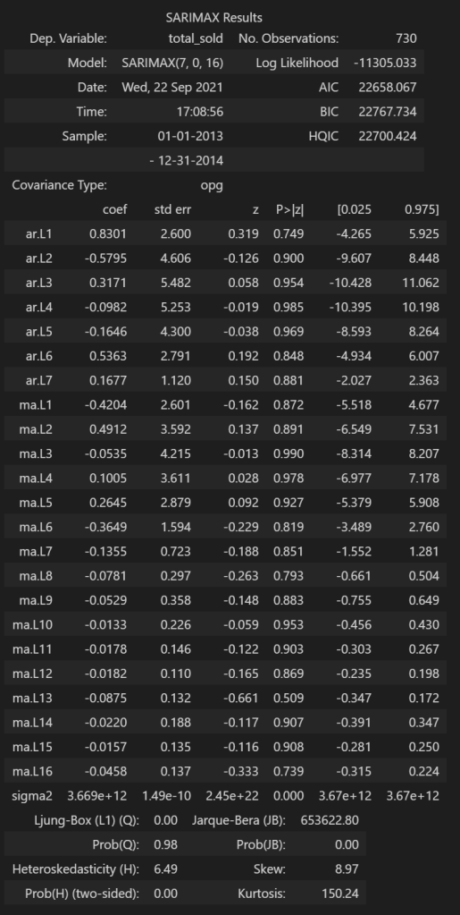
The summary does not look good as the confidence interval includes 0 for all AR and MA coefficients. Next, let’s try grid search using auto_arima() from pmdarima package. I am searching a wide range of
from pmdarima import auto_arima

arima_model = auto_arima(y=df_daily,start_p=1,max_p=30, start_q=1, max_q=60,max_d=5, out_of_sample_size=len(test), scoring='mse')
arima_model.summary()
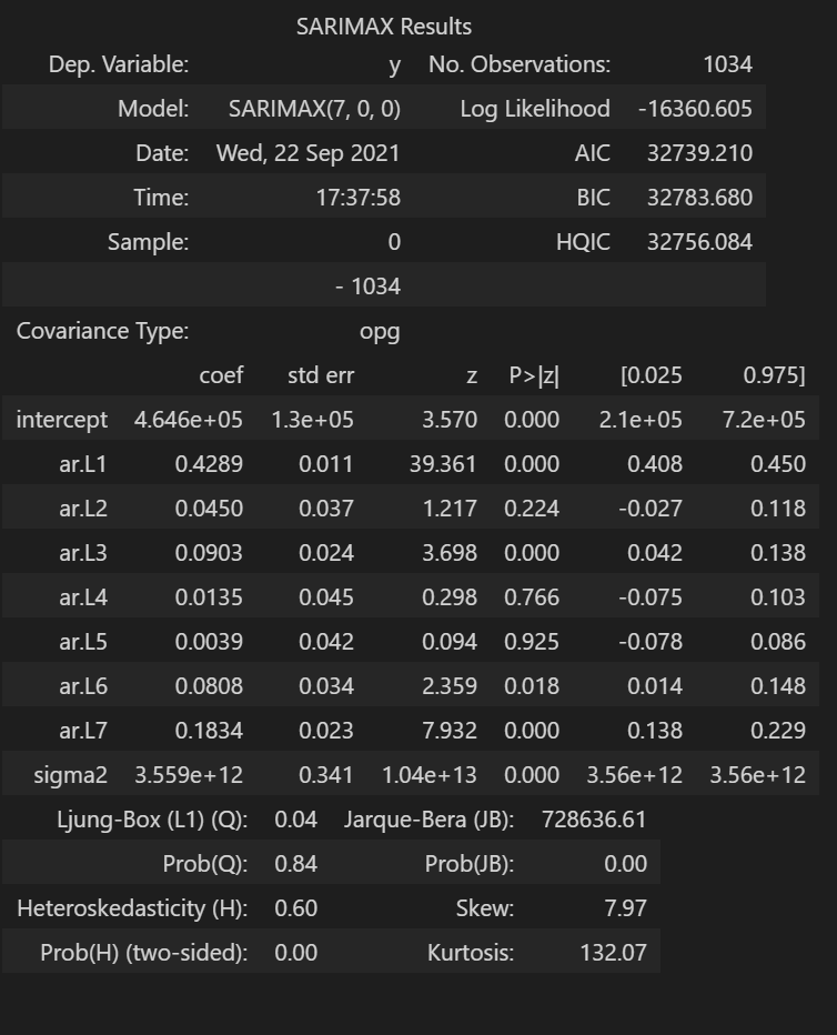
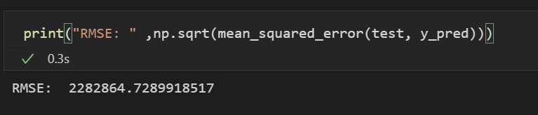
The grid search suggests an ARIMA(7,0,0) model. Let’s fit the training set to the model and calculate the RMSE to compare with previous methods.
from sklearn.metrics import mean_squared_error

model_fit = arima_model.fit(train)
resid = pd.DataFrame(arima_model.resid())
resid.plot(kind='kde')

y_pred = model_fit.predict(len(test), dynamic = True)
print("RMSE: ", np.sqrt(mean_squared_error(test, y_pred)))
And let’ s plot the predicted values vs. actual values.
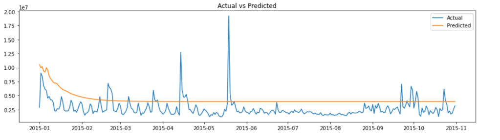
For now, we have applied linear regression, LSTM and ARIMA models to the sales/revenue dataset. Let’s compare the performance of these models measured by RMSE.
- Linear Regression: 3,337,853
- LSTM: 2,712,927
- ARIMA(7,0,0): 2,282,864
It seems ARIMA model has the best performance among all three models. Personally speaking, I would spend more time in constructing and tuning the LSTM model as the current result does not seem to be a true reflection of the capability of an LSTM model.
